Key Features of the Data set

The data set offers rich, structured information about Indigenous-owned businesses in British Columbia. The key fields are:

• Business Name (business_name) – The official name of the business. It serves as the primary identifier for each entry in the data set.

• City (city) – The city or town where the business is physically located.

• Latitude & Longitude (latitude, longitude) – Geographic coordinates that allow for mapping and spatial analysis. Useful for geo visualizations and regional studies.

• Region (region) – A broader classification of the business’s location within British Columbia (e.g., Northeast, Thompson/Okanagan). Helps in regional economic analysis.

• Type (type) – Indicates the business ownership or structure, such as “Private Company,” “Community owned” etc

• Industry Sector (industry_sector) – The NAICS (North American Industry Classification System) code and description that categorize the business’s industry.

• Year Formed (year_formed) – The year the business was established, which can be used to analyze trends in Indigenous entrepreneurship over time.

• Number of Employees (number_of_employees) – A range representing the workforce size, such as “1 to 4” or “5 to 9”. This gives a sense of business scale and economic impact.

Purpose and Use Case

The purpose of this document is to:

• Explore the growth and economic contributions of Indigenous businesses.
• Analyze key challenges and opportunities they face.
• Demonstrate how data can support policy and development decisions.

Case Study

Objective

Which regions in British Columbia have the highest density of Indigenous-owned businesses, and how do industry sectors vary across these clusters?

The goal is to explore the geographic and economic distribution of Indigenous businesses using attributes such as region, city, and industry sector. We apply clustering techniques to identify natural groupings of businesses based on their geo spatial coordinates and sectoral attributes. This helps reveal regional concentrations, uncover potential economic hubs, and provide insights for targeted policy or investment strategies.

Analysis

Loading Libraries

library(diversedata) 
library(tidyverse)  # Loads dplyr, tidyr, stringr, ggplot2, etc.
library(infer)      # For chi-square test
library(dbscan)     # For clustering
library(leaflet)    # For interactive maps
library(treemapify) # For creating treemaps

1. Data Cleaning & Processing

To ensure the quality and consistency of the data set, several pre-processing steps were done:

• Removed records with missing geographic coordinates: These records were excluded since latitude and longitude are crucial for spatial mapping and regional distribution analysis.

• Standardized the format of region names: Region names were converted to title case to ensure consistent grouping and filtering.

• Converted field types: The Industry Sector column was converted to a factor for categorical analysis, and Year Formed was converted to integer to allow for chronological trends and filtering.

# Load and clean the data
indigenousbiz_data <- bcindigenousbiz |>
  filter(!is.na(latitude) & !is.na(longitude)) |>
  mutate(
    region = str_to_title(region),
    industry_sector = as_factor(industry_sector),
    year_formed = as.integer(year_formed)
  )

# Preview cleaned data
indigenousbiz_data |> 
  head()

# A tibble: 6 × 9
  business_name            city  latitude longitude region type  industry_sector
  <chr>                    <chr>    <dbl>     <dbl> <chr>  <chr> <fct>          
1 Ellipsis Energy Inc      Mobe…     55.8     -122. North… Priv… Mining, quarry…
2 Indigenous Community De… Ende…     50.6     -119. Thomp… Priv… Other services…
3 Formline Construction L… Burn…     49.3      123. Lower… Priv… Construction   
4 Quilakwa Investments Lt… Ende…     50.5     -119. Thomp… Comm… Accommodation …
5 Quilakwa Esso            Ende…     50.5     -119. Thomp… Comm… Retail trade   
6 Quilakwa RV Park         Ende…     50.6     -119. Thomp… <NA>  Accommodation …
# ℹ 2 more variables: year_formed <int>, number_of_employees <chr>

2. Exploratory Data Analysis (EDA)

Business count by Region

# Business count by region with tidyverse style
indigenousbiz_data |>
  count(region, sort = TRUE) |>
  ggplot(aes(
    x = fct_reorder(region, n),  # Use forcats for reordering
    y = n,
    fill = n
  )) +
  geom_col() +
  coord_flip() +
  scale_fill_gradient(
    low = "skyblue1",
    high = "skyblue4"
  ) +
  labs(
    title = "Business Count per Region",
    x = "Region",
    y = "Number of Businesses"
  ) +
  theme_minimal()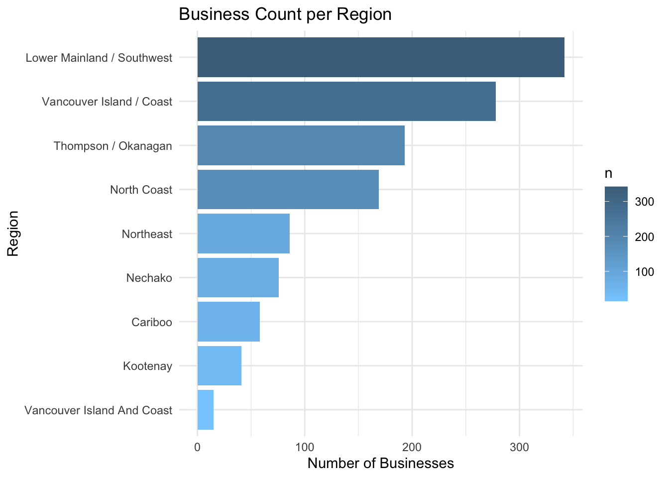

Mapping Businesses

# Create leaflet map
indigenousbiz_data |>
  leaflet() |>
  addTiles() |>
  setView(lng = -125, lat = 54, zoom = 4.6) |>
  addCircleMarkers(
    lng = ~longitude,
    lat = ~latitude,
    label = ~business_name,
    radius = 3,
    color = "#1E90FF",
    stroke = FALSE,
    fillOpacity = 0.7
  )

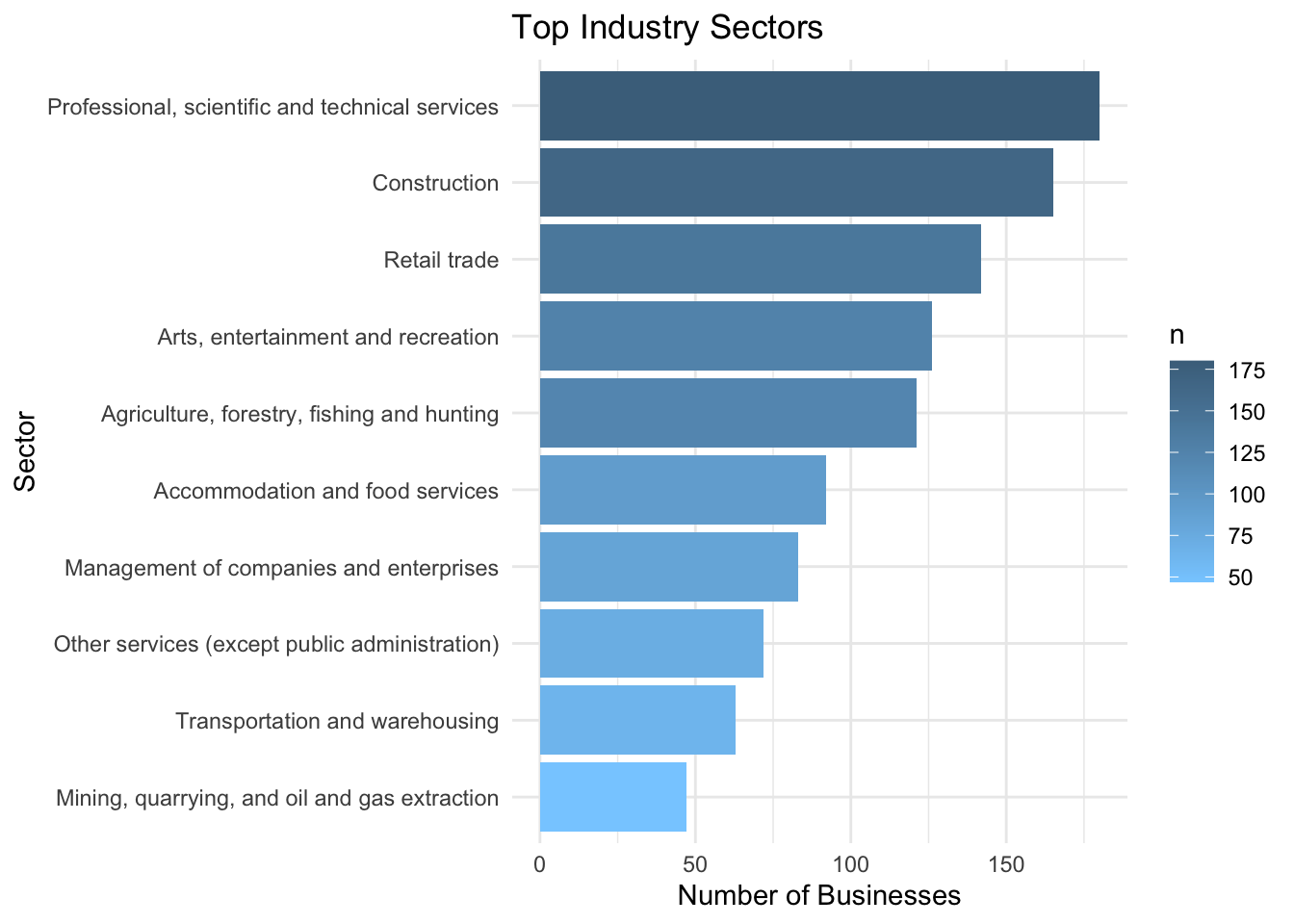
Industry Analysis

3. Chi-Squared Test of Independence

To better understand the relationship between Indigenous business locations and their characteristics, we test whether type (ownership type) is independent of region using a Chi-square test.

Hypotheses

• Null Hypothesis (H₀): Business ownership type and region are independent. That is, the distribution of ownership types is the same across all regions.

• Alternative Hypothesis (Ha): Business ownership type and region are dependent. That is, the distribution of ownership types differs by region.

Chi-squared Assumption Check

• Data in Frequency Form: The data used in this test are raw counts of business records, not percentages or proportions.

• Categorical Variables: Both variables under study, type and region are categorical and represent discrete groups.

• Independence of Observations: Each row in the data set corresponds to a unique business. There is no duplication, satisfying the assumption of independence.

• Expected Count: The Chi-square test expects that all expected cell frequencies are ≥ 5. In our case this assumption is violated.

## Assumptions check

# Step 1: Chi-Square Assumption Check
type_region_table <- table(indigenousbiz_data$type, indigenousbiz_data$region)
chisq_result <- chisq.test(type_region_table)

Warning in chisq.test(type_region_table): Chi-squared approximation may be
incorrect

expected_counts <- chisq_result$expected

min_expected <- min(expected_counts)

cat("Chi-Square Assumptions:\n")

Chi-Square Assumptions:

cat("- Minimum expected count:", round(min_expected, 2), "\n")

- Minimum expected count: 0.01 

if (min_expected >= 5) {
  cat("Chi-squared assumptions met. Proceeding with standard test.\n")
  print(chisq_result)
} else {
  cat("Assumptions violated. Proceeding with simulation-based Chi-squared test.\n\n")
}

Assumptions violated. Proceeding with simulation-based Chi-squared test.

Simulation-based Chi-Square Test with infer

Since the assumption regarding minimum expected cell counts was violated with at least one expected frequency falling below the threshold of 5. The Chi-squared test may yield inaccurate results. To overcome this, we use a simulation-based Chi-squared test via the infer package. This method generates a null distribution by permuting the data under the assumption of independence.

The simulation-based tests still require some assumptions to hold:

- The data must represent independent observations.

• The variables must be categorical.

• The permutations assume that under the null hypothesis, the distribution of values across categories is exchangeable.

# Generate null distribution
null_distribution <- indigenousbiz_data |>
  specify(type ~ region) |>
  hypothesize(null = "independence") |>
  generate(reps = 1000, type = "permute") |>
  calculate(stat = "Chisq")

Warning: Removed 136 rows containing missing values.

# Observed statistic
observed_stat <- indigenousbiz_data |>
  specify(type ~ region) |>
  hypothesize(null = "independence") |>
  calculate(stat = "Chisq")

Warning: Removed 136 rows containing missing values.

# Plot permutation distribution
null_distribution |>
  visualize() +
  shade_p_value(obs_stat = observed_stat, direction = "greater")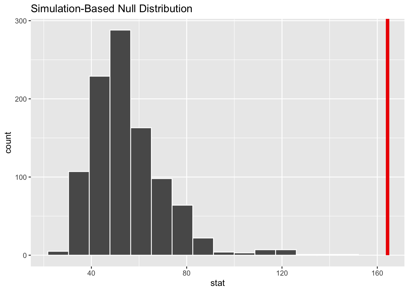

# Compute p-value
p_val <- null_distribution |>
  get_p_value(obs_stat = observed_stat, direction = "greater")

Warning: Please be cautious in reporting a p-value of 0. This result is an approximation
based on the number of `reps` chosen in the `generate()` step.
ℹ See `get_p_value()` (`?infer::get_p_value()`) for more information.

cat("Simulation-based p-value:", round(p_val$p_value, 4), "\n")

Simulation-based p-value: 0 

Inference

To assess whether there is an association between business type and region, we conducted a simulation-based chi-squared test using 1,000 permutations. The null distribution of test statistics generated under the assumption of independence shows that our observed statistic lies far in the tail of the distribution. This suggests that such an extreme result would be highly unlikely if business type and region were truly independent. Therefore, we reject the null hypothesis and conclude that business type and region are statistically dependent.

4. Spatial Clustering of Indigenous Businesses using DBSCAN

To explore geographic patterns in Indigenous business, the technique of clustering based on latitude and longitude coordinates was applied. This analysis revealed several spatial clusters of Indigenous businesses across British Columbia. The treemap provided more information on which were the prominent industries in each cluster.

## DBSCAN Clustering and Leaflet Map

coords <- indigenousbiz_data |>
  select(longitude, latitude) |>
  as.matrix()

set.seed(123)
db <- dbscan::dbscan(coords, eps = 1.2, minPts = 8)

indigenousbiz_data <- indigenousbiz_data |>
  mutate(cluster = factor(db$cluster))

pal <- colorFactor(palette = "Set1", domain = indigenousbiz_data$cluster)

cluster_map <- leaflet(data = indigenousbiz_data) |>
  addTiles() |>
  setView(lng = -125, lat = 54, zoom = 4.6) |>
  addCircleMarkers(
    label = ~business_name,
    radius = 3,
    color = ~pal(cluster),
    stroke = FALSE,
    fillOpacity = 0.7
  ) |>
  addLegend(
    position = "bottomright",
    pal = pal,
    values = ~cluster,
    title = "Cluster",
    opacity = 1
  )

Assuming "longitude" and "latitude" are longitude and latitude, respectively

cluster_map

5. Treemap of Industry sectors within cluster

## Industry Counts and Treemap Visualization

industry_cluster_counts <- indigenousbiz_data |>
  count(cluster, industry_sector)

ranked_industries <- industry_cluster_counts |>
  group_by(cluster) |>
  mutate(rank = rank(-n, ties.method = "min")) |>
  ungroup()

top_industries <- ranked_industries |>
  mutate(
    industry_sector = if_else(rank <= 3, as.character(industry_sector), "Other")
  ) |>
  group_by(cluster, industry_sector) |>
  summarise(n = sum(n), .groups = "drop") |>
  mutate(
    cluster = factor(cluster),
    industry_sector = factor(industry_sector)
  )

ggplot(top_industries, aes(area = n, fill = industry_sector,
                           label = industry_sector, subgroup = cluster)) +
  geom_treemap() +
  geom_treemap_subgroup_border(color = "white") +
  geom_treemap_text(colour = "white", place = "centre", reflow = TRUE) +
  facet_wrap(~ cluster) +
  coord_cartesian(clip = "off") +
  theme(
    legend.position = "none",
    plot.margin = margin(t = 10, r = 10, b = 10, l = 30)
  ) +
  labs(
    title = "Top Industry Sectors by Geo Cluster",
    fill = "Industry Sector"
  )

Warning: Removed 1 row containing missing values or values outside the scale range
(`geom_treemap_text()`).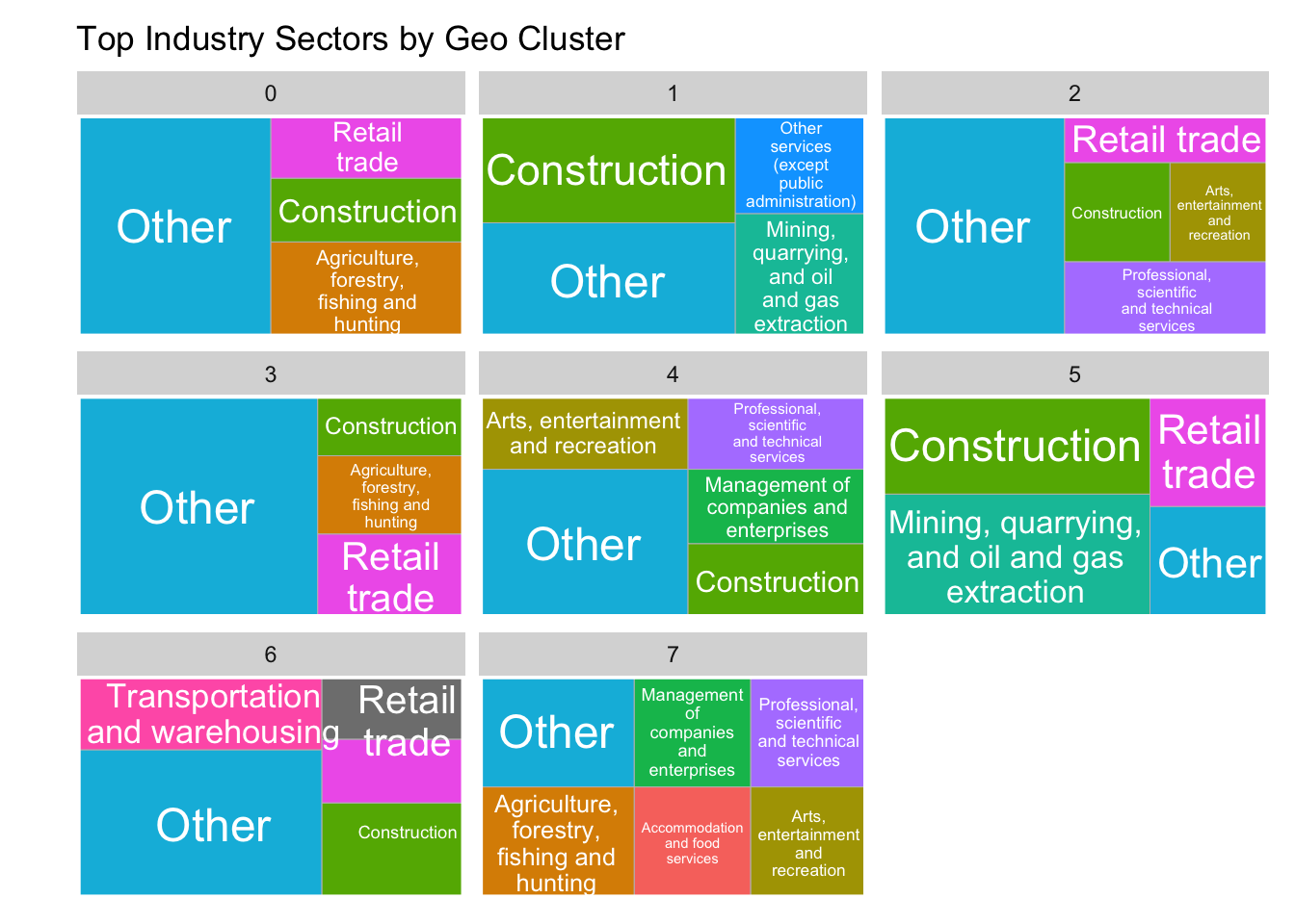

Discussion

This analysis provides a multi faceted view of Indigenous businesses in British Columbia. The statistical and spatial explorations reveal that both regional context and business structure are deeply intertwined with Indigenous entrepreneurship.

The Chi-square test of independence, supported by simulation-based inference due to assumption violations, reveals a statistically significant association between business ownership type and geographic region. This suggests that certain forms of business organization such as community-owned enterprises or private companies may be more prevalent in specific regions, potentially influenced by local governance structures, access to funding, or historical land use patterns.

The spatial clustering using DBSCAN further enriches this narrative by identifying natural groupings of businesses based on their latitude and longitude coordinates. These clusters likely reflect real-world economic and social hubs within the province. The treemap visualization provides a clear breakdown of dominant industry sectors within each spatial cluster, especially after aggregating less-represented sectors into an ‘Other’ category for interpretability.

In summary, this analysis highlights how Indigenous business patterns in British Columbia are shaped by both geographic and organizational factors. While insightful, the findings should be interpreted with caution given the cross-sectional nature of the data and sensitivity of the clustering method.