library(diversedata)
library(tidyverse)  # Loads dplyr, tidyr, stringr, ggplot2, etc.
library(infer)      # For chi-square test
library(dbscan)     # For clustering
library(leaflet)    # For interactive maps
library(treemapify) # For creating treemaps
library(knitr)BC Indigenous Business Listings
NoteTry it live!
Use Binder to explore and run this dataset and analysis interactively in your browser with R. Ideal for students and instructors to run, modify, and test the analysis in a live JupyterLab environment—no setup needed.
About the Data
The BC Indigenous Business Listings data set provides a detailed look at Indigenous-owned businesses operating throughout British Columbia. Compiled in 2025 by the Government of British Columbia and shared under the Open Government Licence - British Columbia, this static data set reflects the state of Indigenous businesses at the time it was created and serves as a vital resource for understanding Indigenous entrepreneurship in the area.
It includes information such as business names, industries, ownership types, and geographic locations, which offers important insights into economic activities within Indigenous communities. This data set showcases the wide ranging participation of Indigenous peoples in the economy, bringing attention to communities that have often been overlooked or underrepresented in traditional business directories and economic plans.
By analyzing this data, policymakers, Indigenous economic development organizations, and researchers can spot geographic trends, industry hubs, and recognize gaps in the system. The data set also sheds light on the distribution of Indigenous businesses across various traditional territories, including urban and rural environments and distinguishing between resource-based and service oriented sectors.
Download
Metadata
CSV Name
bcindigenousbiz.csv
Data set Characteristics
Multivariate
Subject Area
Equity and Diversity
Associated Tasks
Classification, Comparative Analysis, Geo spatial Analysis
Feature Type
Factor, Integer, Numeric
Instances
1259 records
Features
9
Has Missing Values?
Yes
Variables
| Variable Name | Role | Type | Description | Units | Missing Values |
|---|---|---|---|---|---|
| business_name | Feature | Character | Name of the Indigenous business | – | No |
| city | Feature | Character | City or town where the business is located | – | Yes |
| latitude | Feature | Numeric | Latitude coordinate of the business location | Decimal Degrees | Yes |
| longitude | Feature | Numeric | Longitude coordinate of the business location | Decimal Degrees | Yes |
| region | Feature | Factor | Geographical region of British Columbia where the business operates | – | No |
| type | Feature | Factor | Ownership type of the business (e.g., Private, Community Owned, Partnership) | – | Yes |
| industry_sector | Feature | Factor | Industry classification based on NAICS or a similar standard | – | Yes |
| year_formed | Feature | Numeric | Year in which the business was established | Year | Yes |
| number_of_employees | Feature | Factor | Size category representing the number of employees (e.g., “1 to 4”, “10 to 19”) | – | Yes |
Key Features of the Data set
The data set offers rich, structured information about Indigenous-owned businesses in British Columbia. The key fields are:
Business Name (
business_name) – The official name of the business. It serves as the primary identifier for each entry in the data set.City (
city) – The city or town where the business is physically located.Latitude & Longitude (
latitude,longitude) – Geographic coordinates that allow for mapping and spatial analysis. Useful for geo visualizations and regional studies.Region (
region) – A broader classification of the business’s location within British Columbia (e.g., Northeast, Thompson/Okanagan). Helps in regional economic analysis.Type (
type) – Indicates the business ownership or structure, such as “Private Company,” “Community owned” etcIndustry Sector (
industry_sector) – The NAICS (North American Industry Classification System) code and description that categorize the business’s industry.Year Formed (
year_formed) – The year the business was established, which can be used to analyze trends in Indigenous entrepreneurship over time.Number of Employees (
number_of_employees) – A range representing the workforce size, such as “1 to 4” or “5 to 9”. This gives a sense of business scale and economic impact.
Purpose and Use Case
The purpose of this document is to:
- Increase the visibility of Indigenous-owned businesses.
- Provide insights into the distribution, characteristics, and trends of Indigenous businesses in British Columbia.
- Supplemented by community data, study relationships between business presence and community characteristics.
Case Study
Objective
Which regions in British Columbia have the highest density of Indigenous-owned businesses, and how do industry sectors vary across these clusters?
The goal is to explore the geographic and economic distribution of Indigenous businesses using attributes such as region, city, and industry sector. We apply clustering techniques to identify natural groupings of businesses based on their geospatial coordinates and sectoral attributes. This helps highlight regional concentrations, suggest potential areas of economic activity, and offer insights that could inform future policy or investment considerations.
Analysis
Loading Libraries
import diversedata as dd
import numpy as np
import pandas as pd
import altair as alt
import plotly.express as px
from scipy.stats import chi2_contingency
from sklearn.cluster import DBSCAN
from IPython.display import Markdown
np.random.seed(123) # set seed for reproducibility
1. Data Cleaning & Processing
To ensure the quality and consistency of the data set, several pre-processing steps were done:
Removed records with missing geographic coordinates: These records were excluded since latitude and longitude are crucial for spatial mapping and regional distribution analysis.
Standardized the format of region names: Region names were converted to title case to ensure consistent grouping and filtering.
Converted field types: The
Industry Sectorcolumn was converted to a factor for categorical analysis, andYear Formedwas converted to integer to allow for chronological trends and filtering.
# Load and clean the data
indigenousbiz_data <- bcindigenousbiz |>
  filter(!is.na(latitude) & !is.na(longitude)) |>
  mutate(
    region = str_to_title(region),
    industry_sector = as_factor(industry_sector),
    year_formed = as.integer(year_formed)
  )

# Preview cleaned data
indigenousbiz_data |>
  head() |>
kable()| business_name | city | latitude | longitude | region | type | industry_sector | year_formed | number_of_employees |
|---|---|---|---|---|---|---|---|---|
| Ellipsis Energy Inc | Moberly Lake | 55.81937 | -121.8346 | Northeast | Private Company | Mining, quarrying, and oil and gas extraction | 2012 | 5 to 9 |
| Indigenous Community Development & Prosperity (ICDPRO) | Enderby | 50.55150 | -119.1335 | Thompson / Okanagan | Private Company | Other services (except public administration) | 2020 | 1 to 4 |
| Formline Construction Ltd. | Burnaby | 49.26605 | 123.0058 | Lower Mainland / Southwest | Private Company | Construction | 2021 | 1 to 4 |
| Quilakwa Investments Ltd. | Enderby | 50.53751 | -119.1420 | Thompson / Okanagan | Community Owned Company | Accommodation and food services | 1984 | 20 to 49 |
| Quilakwa Esso | Enderby | 50.53751 | -119.1420 | Thompson / Okanagan | Community Owned Company | Retail trade | 1984 | 10 to 19 |
| Quilakwa RV Park | Enderby | 50.55150 | -119.1335 | Thompson / Okanagan | NA | Accommodation and food services | 1984 | 1 to 4 |
# Load and clean the data
indigenousbiz_data = dd.load_data("bcindigenousbiz")
indigenousbiz_data = indigenousbiz_data.dropna(subset=["latitude", "longitude"])
indigenousbiz_data["region"] = indigenousbiz_data["region"].str.title()
indigenousbiz_data["industry_sector"] = pd.Categorical(
    indigenousbiz_data["industry_sector"], ordered=False
)
indigenousbiz_data["year_formed"] = indigenousbiz_data["year_formed"].astype("Int64")

# Preview cleaned data
Markdown(indigenousbiz_data.head().to_markdown())| business_name | city | latitude | longitude | region | type | industry_sector | year_formed | number_of_employees | |
|---|---|---|---|---|---|---|---|---|---|
| 0 | Ellipsis Energy Inc | Moberly Lake | 55.8194 | -121.835 | Northeast | Private Company | Mining, quarrying, and oil and gas extraction | 2012 | 5 to 9 |
| 1 | Indigenous Community Development & Prosperity (ICDPRO) | Enderby | 50.5515 | -119.134 | Thompson / Okanagan | Private Company | Other services (except public administration) | 2020 | 1 to 4 |
| 2 | Formline Construction Ltd. | Burnaby | 49.2661 | 123.006 | Lower Mainland / Southwest | Private Company | Construction | 2021 | 1 to 4 |
| 3 | Quilakwa Investments Ltd. | Enderby | 50.5375 | -119.142 | Thompson / Okanagan | Community Owned Company | Accommodation and food services | 1984 | 20 to 49 |
| 4 | Quilakwa Esso | Enderby | 50.5375 | -119.142 | Thompson / Okanagan | Community Owned Company | Retail trade | 1984 | 10 to 19 |
2. Exploratory Data Analysis (EDA)
Business count by Region
# Business count by region with tidyverse style
indigenousbiz_data |>
  count(region, sort = TRUE) |>
  ggplot(aes(
    x = fct_reorder(region, -n),  # Use forcats for reordering
    y = n,
  )) +
  geom_col(fill = 'skyblue') +
  coord_flip() +
  labs(
    title = "Business Count per Region",
    x = "Region",
    y = "Number of Businesses"
  ) +
  theme_minimal()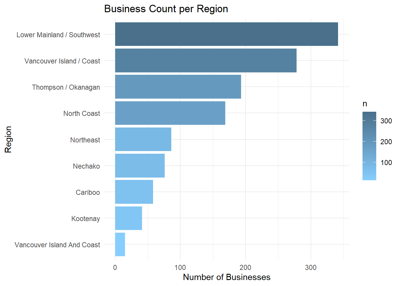
alt.Chart(indigenousbiz_data).mark_bar().encode(
    x=alt.X("count()").title("Number of Businesses"),
    y=alt.Y("region").sort("x").title("Region"),
).properties(title="Business Count per Region", width=500, height=300)
Mapping Businesses
# Create leaflet map
indigenousbiz_data |>
  leaflet() |>
  addTiles() |>
  setView(lng = -125, lat = 54.5, zoom = 4.5) |>
  addCircleMarkers(
    lng = ~longitude,
    lat = ~latitude,
    label = ~business_name,
    radius = 3,
    color = "#1E90FF",
    stroke = FALSE,
    fillOpacity = 0.7
  )
fig_map = px.scatter_map(
indigenousbiz_data,
lat="latitude",
lon="longitude",
opacity=0.5,
zoom=4,
center={"lat": 54.5, "lon": -128},
hover_name="business_name"
)
fig_map = fig_map.update_layout(
margin=dict(l=0, r=0, t=30, b=10),
width=700,
height=550,
mapbox_style="open-street-map"
)Industry Analysis
# Plot top 10 industry sectors
indigenousbiz_data |>
  count(industry_sector, sort = TRUE) |>
  slice_max(n, n = 10) |>
  ggplot(aes(
    x = fct_reorder(industry_sector, -n),
    y = n,
  )) +
  geom_col(fill = 'skyblue') +
  coord_flip() +
  labs(
    title = "Top Industry Sectors",
    x = "Sector",
    y = "Number of Businesses"
  ) +
  theme_minimal()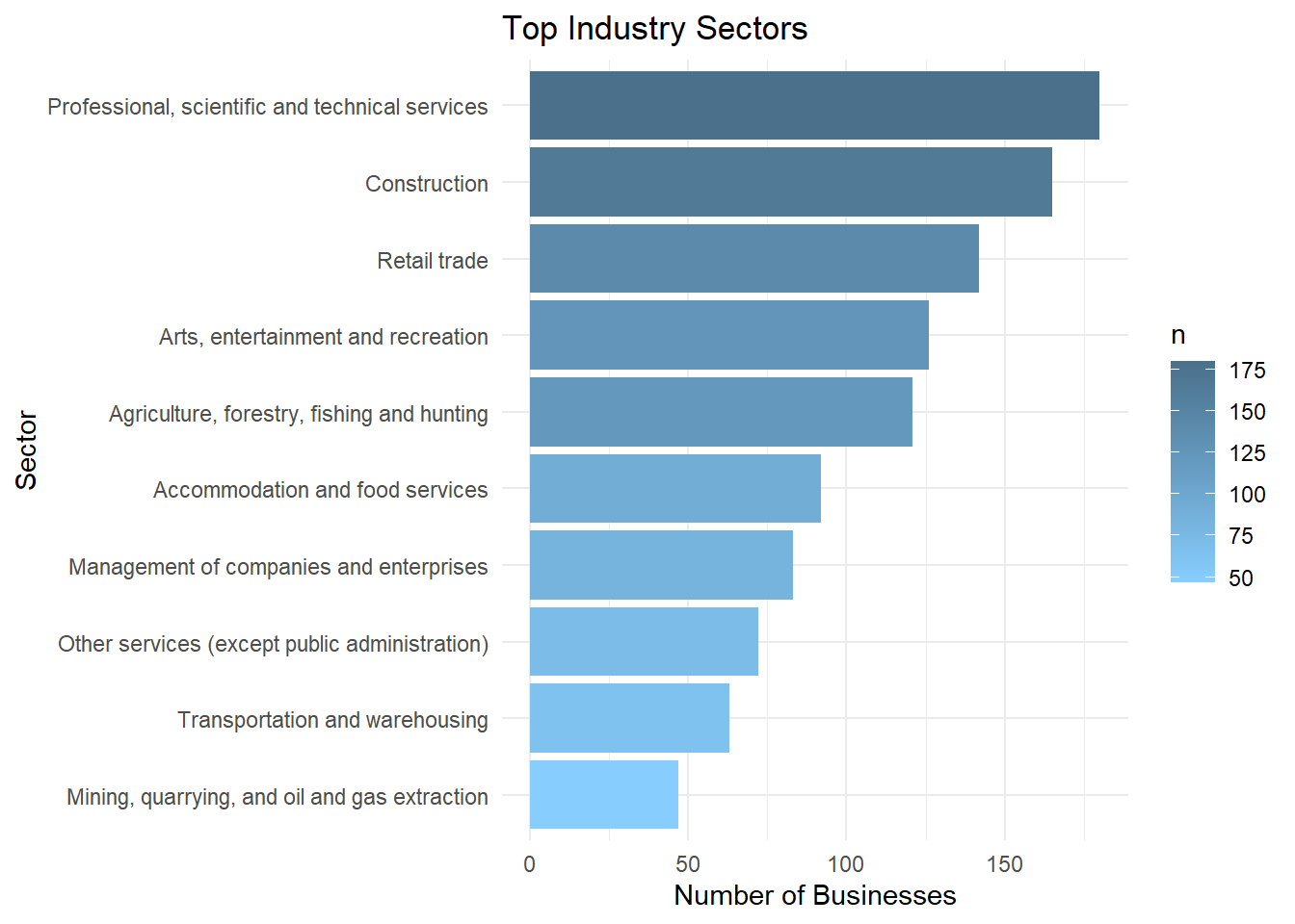
top_10_sectors = (
    indigenousbiz_data.groupby("industry_sector", observed=True)
    .size()
    .reset_index(name="count")
    .sort_values(by="count", ascending=False)
    .head(10)
)

alt.Chart(top_10_sectors).mark_bar().encode(
    x=alt.X("count").title("Number of Businesses"),
    y=alt.Y("industry_sector").sort("x").title("Sector").axis(alt.Axis(labelLimit=300))
).properties(title="Top Industry Sectors", width=500, height=300)
3. Chi-Squared Test of Independence
To better understand the relationship between Indigenous business locations and their characteristics, we test whether type (ownership type) is independent of region using a Chi-square test.
Hypotheses
Null Hypothesis (H₀): Business ownership type and region are independent. That is, the distribution of ownership types is the same across all regions.
Alternative Hypothesis (Ha): Business ownership type and region are dependent. That is, the distribution of ownership types differs by region.
Chi-squared Assumption Check
Data in Frequency Form: The data used in this test are raw counts of business records, not percentages or proportions.
Categorical Variables: Both variables under study, type and region are categorical and represent discrete groups.
Independence of Observations: Each row in the data set corresponds to a unique business. There is no duplication, satisfying the assumption of independence.
Expected Count: The Chi-square test expects that all expected cell frequencies are ≥ 5. In our case this assumption is violated.
## Assumptions check

# Step 1: Chi-Square Assumption Check
type_region_table <- table(indigenousbiz_data$type, indigenousbiz_data$region)
chisq_result <- chisq.test(type_region_table)
expected_counts <- chisq_result$expected

min_expected <- min(expected_counts)

cat("Chi-Square Assumptions Check:\n")
cat("- Minimum expected count:", round(min_expected, 2), "\n")

if (min_expected >= 5) {
  cat("Chi-squared assumptions met. Proceeding with standard test.\n")
  print(chisq_result)
} else {
  cat("Assumptions violated. Proceeding with simulation-based Chi-squared test.\n\n")
}
Chi-Square Assumptions Check:
- Minimum expected count: 0.01
Assumptions violated. Proceeding with simulation-based Chi-squared test.type_region_table = pd.crosstab(
indigenousbiz_data["type"], indigenousbiz_data["region"]
)
chi2_stat, p_value, dof, expected = chi2_contingency(type_region_table)
min_expected = expected.min()
print("Chi-Square Assumptions Check:")
print(f"- Minimum expected count: {min_expected:.2f}")
if min_expected >= 5:
print("Chi-squared assumptions met. Proceeding with standard test.")
print(f"Chi2 Statistic: {chi2_stat}")
print(f"P-value: {p_value}")
print(f"Degrees of Freedom: {dof}")
else:
print("Assumptions violated. Proceeding with simulation-based Chi-squared test.")Chi-Square Assumptions Check:
- Minimum expected count: 1.76
Assumptions violated. Proceeding with simulation-based Chi-squared test.Simulation-based Chi-Square Test with infer
Since the assumption regarding minimum expected cell counts was violated with at least one expected frequency falling below the threshold of 5. The Chi-squared test may yield inaccurate results. To overcome this, we use a simulation-based Chi-squared test via the infer package. This method generates a null distribution by permuting the data under the assumption of independence.
The simulation-based tests still require some assumptions to hold:
The data must represent independent observations.
The variables must be categorical.
The permutations assume that under the null hypothesis, the distribution of values across categories is exchangeable.
# Generate null distribution
null_distribution <- indigenousbiz_data |>
  specify(type ~ region) |>
  hypothesize(null = "independence") |>
  generate(reps = 1000, type = "permute") |>
  calculate(stat = "Chisq")

# Observed statistic
observed_stat <- indigenousbiz_data |>
  specify(type ~ region) |>
  hypothesize(null = "independence") |>
  calculate(stat = "Chisq")

# Plot permutation distribution
null_distribution |>
  visualize() +
  shade_p_value(obs_stat = observed_stat, direction = "greater")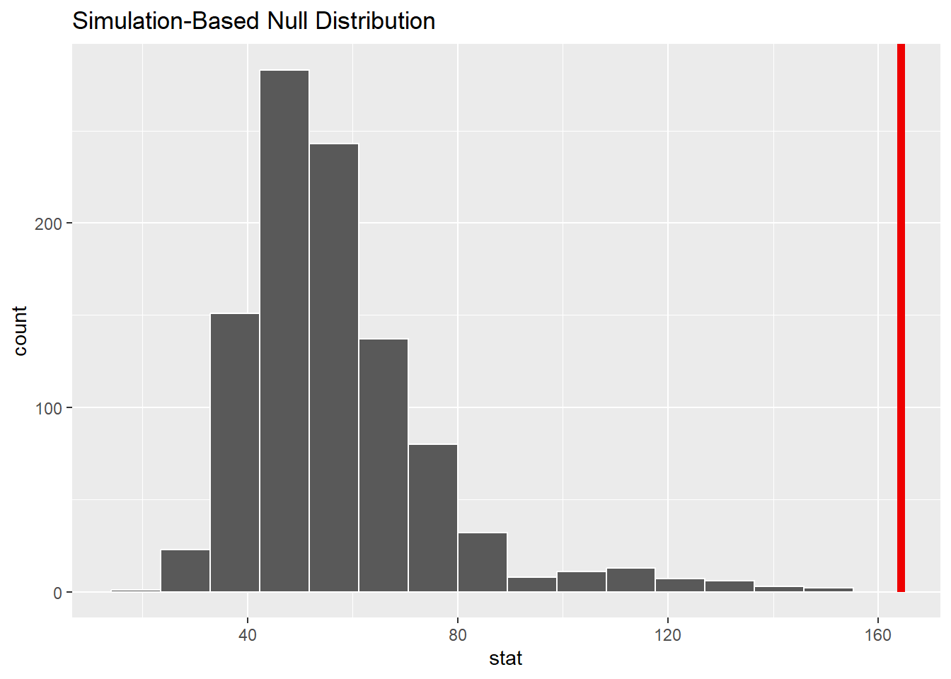
# Compute p-value
p_val <- null_distribution |>
  get_p_value(obs_stat = observed_stat, direction = "greater")

cat("Simulation-based p-value:", round(p_val$p_value, 4), "\n")
Simulation-based p-value: 0 # Drop missing values in the columns of interest
df = indigenousbiz_data.dropna(subset=["type", "region"])
# Make function to calculate chi-square stat
def chi2_statistic(data):
table = pd.crosstab(data["type"], data["region"])
chi2, _, _, _ = chi2_contingency(table)
return chi2
# Generate null distribution
reps = 1000
null_distribution = []
for rep in range(reps):
shuffled = df.copy()
shuffled["region"] = np.random.permutation(shuffled["region"])
null_distribution.append(chi2_statistic(shuffled))
null_distribution = np.array(null_distribution)
null_df = pd.DataFrame({"chi2_stat": null_distribution})
# Observed statistic from earlier
observed_stat = chi2_stat
# Plot permutation distribution
histogram = alt.Chart(null_df).mark_bar(color="grey").encode(
x=alt.X("chi2_stat:Q").bin(alt.Bin(maxbins=30)).title("Chi-square statistic"),
y=alt.Y("count()").title("Count")
).properties(width=600, height=400, title="Simulation-based Null Distribution")
observed_stat_line = alt.Chart(pd.DataFrame({"obs": [observed_stat]})).mark_rule(color="red", size=3).encode(
x="obs:Q"
)
permutation_dist = histogram + observed_stat_line
permutation_dist# Compute p-value (proportion of null stats >= observed stat)
p_value = np.mean(null_distribution >= observed_stat)
print(f"Simulation-based p-value: {p_value:.4e}")Simulation-based p-value: 0.0000e+00Inference
To assess whether there is an association between business type and region, we conducted a simulation-based chi-squared test using 1,000 permutations. The null distribution of test statistics generated under the assumption of independence shows that our observed statistic lies far in the tail of the distribution. This suggests that such an extreme result would be highly unlikely if business type and region were truly independent. Therefore, we reject the null hypothesis and conclude that business type and region are statistically dependent.
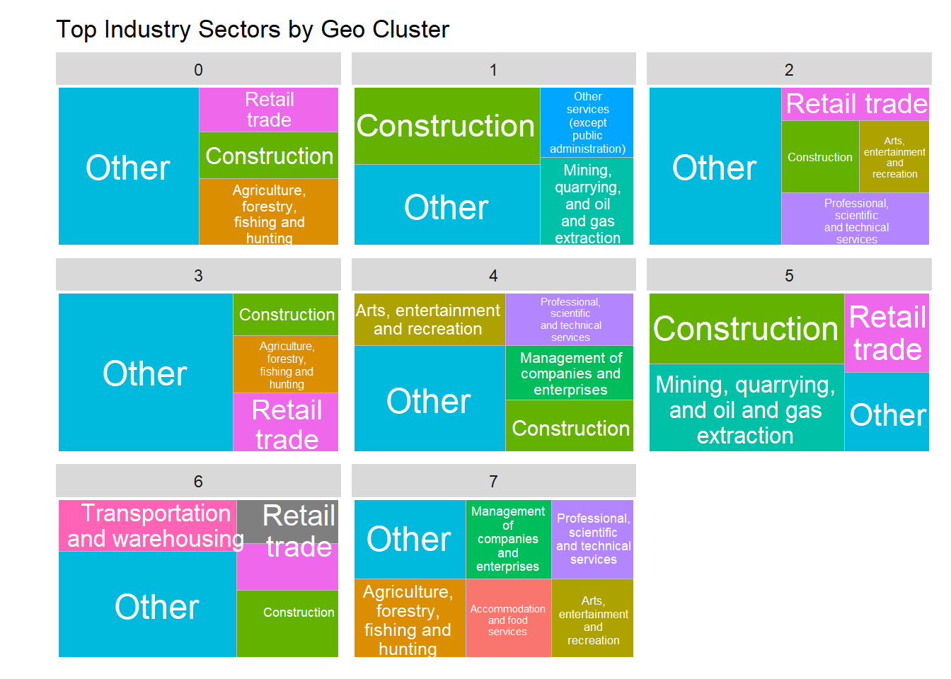
4. Spatial Clustering of Indigenous Businesses using DBSCAN
To explore geographic patterns in Indigenous business, the technique of clustering based on latitude and longitude coordinates was applied. This analysis revealed several spatial clusters of Indigenous businesses across British Columbia. The treemap provided more information on which were the prominent industries in each cluster.
## DBSCAN Clustering and Leaflet Map

coords <- indigenousbiz_data |>
  select(longitude, latitude) |>
  as.matrix()

set.seed(123)
db <- dbscan::dbscan(coords, eps = 1.2, minPts = 8)

indigenousbiz_data <- indigenousbiz_data |>
  mutate(cluster = factor(db$cluster))

pal <- colorFactor(palette = "Set1", domain = indigenousbiz_data$cluster)

cluster_map <- leaflet(data = indigenousbiz_data) |>
  addTiles() |>
  setView(lng = -125, lat = 54.5, zoom = 4.5) |>
  addCircleMarkers(
    label = ~business_name,
    radius = 3,
    color = ~pal(cluster),
    stroke = FALSE,
    fillOpacity = 0.7
  ) |>
  addLegend(
    position = "bottomright",
    pal = pal,
    values = ~cluster,
    title = "Cluster",
    opacity = 1
  )

cluster_map
db = DBSCAN(eps=1.2, min_samples=8).fit(indigenousbiz_data[["longitude", "latitude"]])
# add cluster labels as new column to the data
indigenousbiz_data["cluster"] = db.labels_.astype(str)
# visualize on map
fig_cluster_map = px.scatter_map(
indigenousbiz_data,
lat="latitude",
lon="longitude",
color="cluster",
opacity=0.5,
zoom=4,
center={"lat": 54.5, "lon": -128},
hover_name="business_name",
)
fig_cluster_map = fig_cluster_map.update_layout(
margin=dict(l=0, r=0, t=30, b=10),
width=700,
height=550,
mapbox_style="open-street-map"
)5. Treemap of Industry sectors within cluster
## Industry Counts and Treemap Visualization

industry_cluster_counts <- indigenousbiz_data |>
  count(cluster, industry_sector)

ranked_industries <- industry_cluster_counts |>
  group_by(cluster) |>
  mutate(rank = rank(-n, ties.method = "min")) |>
  ungroup()

top_industries <- ranked_industries |>
  mutate(
    industry_sector = if_else(rank <= 3, as.character(industry_sector), "Other")
  ) |>
  group_by(cluster, industry_sector) |>
  summarise(n = sum(n), .groups = "drop") |>
  mutate(
    cluster = factor(cluster),
    industry_sector = factor(industry_sector)
  )

ggplot(top_industries, aes(area = n, fill = industry_sector,
                           label = industry_sector, subgroup = cluster)) +
  geom_treemap() +
  geom_treemap_subgroup_border(color = "white") +
  geom_treemap_text(colour = "white", place = "centre", reflow = TRUE) +
  facet_wrap(~ cluster) +
  coord_cartesian(clip = "off") +
  theme(
    legend.position = "none",
    plot.margin = margin(t = 10, r = 10, b = 10, l = 30)
  ) +
  labs(
    title = "Top Industry Sectors by Geo Cluster",
    fill = "Industry Sector"
  )
industry_cluster_counts = (
    indigenousbiz_data.groupby(by=["cluster", "industry_sector"], observed=True)
    .size()
    .reset_index(name="n")
)

industry_cluster_counts["rank"] = industry_cluster_counts.groupby(
    by="cluster", observed=True
)["n"].rank(method="min", ascending=False)

industry_cluster_counts["industry_sector_label"] = industry_cluster_counts.apply(
    lambda row: row["industry_sector"] if row["rank"] <= 3 else "Other", axis=1
)

top_industries = (
    industry_cluster_counts.groupby(
        by=["cluster", "industry_sector_label"], observed=True
    )
    .agg({"n": "sum"})
    .reset_index()
)

top_industries["hover_text"] = (
    "Cluster: "
    + top_industries["cluster"].astype(str)
    + "<br>Industry: "
    + top_industries["industry_sector_label"].astype(str)
    + "<br>Businesses: "
    + top_industries["n"].astype(str)
)

fig_treemap = px.treemap(
    top_industries,
    path=["cluster", "industry_sector_label"],
    values="n",
    color="industry_sector_label",
    custom_data=["hover_text"],
    title="Top Industry Sectors by Geo Cluster",
)

fig_treemap = fig_treemap.update_traces(
    textinfo="label+value", hovertemplate="%{customdata[0]}<extra></extra>"
)

fig_treemap = fig_treemap.update_layout(margin=dict(l=10, r=10, t=30, b=10))
Note
The R and Python cluster labels differ.
Discussion
This analysis provides a multi faceted view of Indigenous businesses in British Columbia. The statistical and spatial explorations reveal that both regional context and business structure are deeply intertwined with Indigenous entrepreneurship.
The Chi-square test of independence, supported by simulation-based inference due to assumption violations, reveals a statistically significant association between business ownership type and geographic region. This suggests that certain forms of business organization such as community-owned enterprises or private companies may be more prevalent in specific regions, potentially influenced by local governance structures, access to funding, or historical land use patterns.
The spatial clustering using DBSCAN further enriches this narrative by identifying natural groupings of businesses based on their latitude and longitude coordinates. These clusters likely reflect real-world economic and social hubs within the province. The treemap visualization provides a clear breakdown of dominant industry sectors within each spatial cluster, especially after aggregating less-represented sectors into an ‘Other’ category for interpretability.
In summary, this analysis highlights how Indigenous business patterns in British Columbia are shaped by both geographic and organizational factors. While insightful, the findings should be interpreted with caution given the cross-sectional nature of the data and sensitivity of the clustering method.
Attribution
Data sourced from the Government of British Columbia via the Government of Canada’s Open Government Portal, available under an Open Government Licence – British Columbia. Original data set: BC Indigenous Business Listings.